Integration as an Inner Product

Quadrature in Value Space¶

The quadrature framework is simple. Sample $f$ at nodes $x_0, \ldots, x_n$, build the Lagrange interpolant $p_n = \sum_j f_j\, \ell_j$, and integrate:

The continuous integral has become a finite-dimensional inner product: the value vector $\mathbf{f}$ tested against the weight vector $\mathbf{w}$. Once the nodes are fixed, the quadrature weights $w_j = \int_{-1}^1 \ell_j(x)\, dx$ are purely geometric and can be computed once and reused for any $f$.

Trapezoidal uses the hat basis on an equispaced grid and gets the familiar weights $w_j = h$ (with $h/2$ at the endpoints). Newton-Cotes generalises this to higher-degree polynomial interpolation on equispaced nodes, but as in §2 it suffers from Runge at large $n$. The weights start to alternate in sign and grow exponentially, turning the sum into catastrophic cancellation. Don’t go that route.

Chebyshev nodes fix it, as always. On them the integrals $w_j = \int_{-1}^{1} \ell_j(x)\, dx$ are bounded and positive. Computing them directly from the barycentric form of $\ell_j$ is cumbersome, but we already have the right machinery. In the next section we expand $p_n$ in the Chebyshev basis and integrate there; afterwards we translate back to read off the explicit weights.

Integration in Coefficient Space¶

Expand $p_n$ in the Chebyshev basis

and integrate term by term using linearity:

Everything reduces to the closed-form values of $\int T_k$, which come cleanly out of the $x = \cos\theta$ substitution.

Plugging the proposition into the term-by-term sum collapses the integral of $p_n$ to a clean one-liner:

Only the even-index Chebyshev coefficients contribute. Operationally: compute $\mathbf{c} = \mathrm{DCT}(\mathbf{f})$ in $O(N \log N)$, then dot it against the integral vector $\mathbf{I} = (I_0, I_1, \ldots, I_N) = (2, 0, -\tfrac{2}{3}, 0, -\tfrac{2}{15}, 0, -\tfrac{2}{35}, \ldots)$ from Proposition 1.

Clenshaw-Curtis: Back to Value-Space Weights¶

Chaining the two views gives the value-space weights we promised. Writing $I_k = \int_{-1}^1 T_k$ for the integrals from Proposition 1, the coefficient-space integral is

From Where to Place the Nodes the discrete Chebyshev coefficients are

where $\sum''$ halves the $j = 0$ and $j = N$ terms. Substituting this into the coefficient-space integral,

and swapping the order of summation,

The inner sum in brackets defines the Clenshaw-Curtis weights. Only the even $k$ contribute, since $I_k = 0$ for $k$ odd. So

with an extra factor of $1/2$ at the endpoints $j = 0, N$ coming from the outer $\sum''$. The closed form is a finite cosine series in $j$; evaluating it at $j = 0, 1, \ldots, N$ produces the whole weight vector in $O(N^2)$ work, or $O(N \log N)$ with an FFT.

Source

import numpy as np
import matplotlib.pyplot as plt
import scipy.fft as fft

def chebpts(N):
    return np.cos(np.pi * np.arange(N+1) / N)

def cc_weights(N):
    """Clenshaw-Curtis weights on Chebyshev points x_j = cos(j*pi/N),
    from Trefethen's clencurt.m."""
    theta = np.pi * np.arange(N+1) / N
    w = np.zeros(N+1)
    v = np.ones(N-1)
    if N % 2 == 0:
        w[0] = 1.0 / (N**2 - 1); w[N] = w[0]
        for k in range(1, N//2):
            v -= 2 * np.cos(2*k*theta[1:N]) / (4*k**2 - 1)
        v -= np.cos(N*theta[1:N]) / (N**2 - 1)
    else:
        w[0] = 1.0 / N**2; w[N] = w[0]
        for k in range(1, (N-1)//2 + 1):
            v -= 2 * np.cos(2*k*theta[1:N]) / (4*k**2 - 1)
    w[1:N] = 2 * v / N
    return w

N = 32
w = cc_weights(N); x = chebpts(N)
fig, ax = plt.subplots(figsize=(7, 3.8))
ax.stem(np.arange(N+1), w, basefmt=' ')
ax.set_xlabel('node index $j$'); ax.set_ylabel('$w_j$')
ax.set_title(f'Clenshaw-Curtis weights, $N = {N}$ (all positive)')
plt.tight_layout(); plt.show()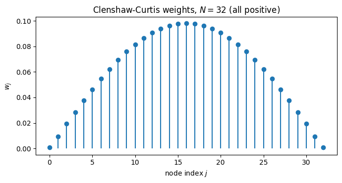

All weights are positive, so the quadrature never relies on delicate sign cancellation. The endpoint weights are small to compensate for the endpoint clustering of Chebyshev nodes: each node sits in a region of size $\propto 1/N$ in the interior and $\propto 1/N^2$ near $\pm 1$, and the weights mirror that. Contrast with Newton-Cotes at large $N$, where weights alternate sign and grow exponentially.

Convergence¶

The quadrature error inherits the truncation error of the Chebyshev expansion, so the rates from Regularity and Coefficient Decay translate directly.

Source

from scipy.special import erf

def trapezoid(f, N):
    x = np.linspace(-1, 1, N+1); h = x[1] - x[0]
    fx = f(x)
    return h * (fx[0]/2 + fx[-1]/2 + fx[1:-1].sum())

def cc(f, N):
    x = chebpts(N); return cc_weights(N) @ f(x)

# (a) Analytic integrand
f1 = lambda x: np.exp(-x**2)
I1 = np.sqrt(np.pi) * erf(1.0)

# (b) C^2 integrand: |x|^3
f2 = lambda x: np.abs(x)**3
I2 = 0.5

Ns = 2**np.arange(2, 11)
err_t1 = [abs(trapezoid(f1, N) - I1) for N in Ns]
err_c1 = [abs(cc(f1, N)        - I1) for N in Ns]
err_t2 = [abs(trapezoid(f2, N) - I2) for N in Ns]
err_c2 = [abs(cc(f2, N)        - I2) for N in Ns]

fig, (ax1, ax2) = plt.subplots(1, 2, figsize=(10, 4))
ax1.loglog(Ns, err_t1, 'o-', label='trapezoid')
ax1.loglog(Ns, err_c1, 's-', label='Clenshaw-Curtis')
ax1.set_title(r'analytic: $\int_{-1}^{1} e^{-x^2} dx$')
ax1.set_xlabel('$N$'); ax1.set_ylabel('error'); ax1.legend()

ax2.loglog(Ns, err_t2, 'o-', label='trapezoid')
ax2.loglog(Ns, err_c2, 's-', label='Clenshaw-Curtis')
ax2.loglog(Ns, 1.0/Ns**4, 'k:', label=r'$N^{-4}$')
ax2.set_title(r'$C^2$: $\int_{-1}^{1} |x|^3 dx$')
ax2.set_xlabel('$N$'); ax2.legend()
plt.tight_layout(); plt.show()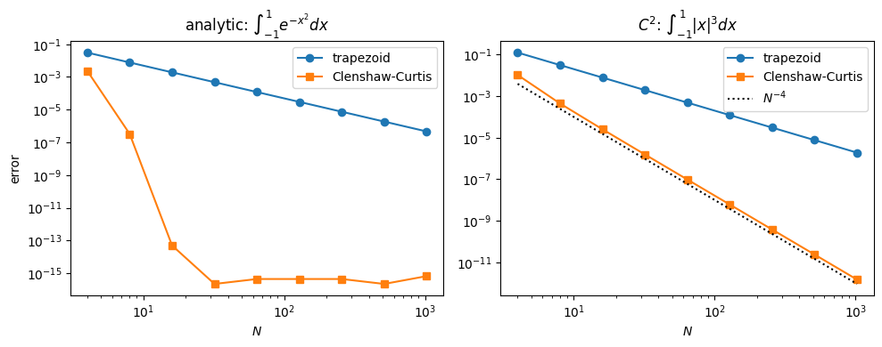

The analytic integrand drops to machine precision around $N \approx 30$ under Clenshaw-Curtis; trapezoid plods along at $O(N^{-2})$. For the $C^2$ integrand both rules eventually drop algebraically, but Clenshaw-Curtis benefits from each extra derivative the integrand has, while trapezoid is permanently stuck at second order.

A Demo¶

Try the rule on something genuinely awful. The integrand

oscillates 40 times across $[-1,1]$, has an envelope that itself rides on $e^x$, and admits no closed-form antiderivative. It is, however, real-analytic on $[-1,1]$, so the regularity dictionary predicts geometric convergence once the resolution is high enough to see the oscillation.

Source

def g(x):
    return np.exp(x) * np.cosh(4*np.sin(40*x))**(-np.exp(x))

xx = np.linspace(-1, 1, 4000)
fig, axes = plt.subplots(1, 2, figsize=(11, 4))
axes[0].plot(xx, g(xx), 'C2', lw=0.6)
axes[0].set_xlabel('$x$')
axes[0].set_title(r"$g(x) = e^x [\mathrm{sech}(4\sin 40x)]^{e^x}$")

I_ref = cc(g, 4096)
Ns = 2**np.arange(4, 13)
err_cc    = [abs(cc(g, N)        - I_ref) for N in Ns]
err_trapz = [abs(trapezoid(g, N) - I_ref) for N in Ns]

axes[1].loglog(Ns, err_cc,    'o-', label='Clenshaw-Curtis')
axes[1].loglog(Ns, err_trapz, 's-', label='trapezoid')
axes[1].set_xlabel('$N$'); axes[1].set_ylabel(r'error vs. $I_{4096}$')
axes[1].set_title('Convergence on the wild integrand')
axes[1].legend()
plt.tight_layout(); plt.show()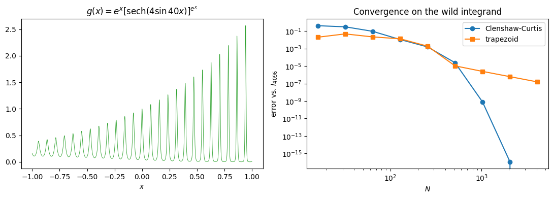

Two regimes, separated by a knee where Clenshaw-Curtis finally resolves the $\sin(40x)$ oscillation. Below the knee the integrand looks rougher than $\mathbb{P}_N$ can capture and both rules flounder. Above it, Clenshaw-Curtis switches to its asymptotic geometric rate and reaches machine precision within a handful of doublings. Trapezoid, blind to the analyticity, plods on at $O(N^{-2})$ throughout.

The take-away: spectral convergence is a promise about the asymptotic regime, contingent on resolving whatever oscillations the integrand already has. Once you cross that threshold, the difference between the two rules is no longer a constant factor. It is the difference between “correct to all digits” and “still wrong in the second.”