Globalization Strategies - Introduction to Scientific Computing

Big Idea

Newton’s method converges quadratically, but only if you start close enough. Globalization modifies Newton to converge from farther away by controlling step sizes. The two main approaches differ in what they monitor: the residual $\|\mathbf{F}(\mathbf{x})\|$ (backward error) or the Newton correction $\|\Delta\mathbf{x}\|$ (forward error estimate).

The Problem with Pure Newton¶

Newton’s method has a fundamental tension:

Near the solution: quadratic convergence, take the full Newton step.
Far from the solution: the linear model may be poor, and the full step could make things worse.

Example 1 (Newton Diverging)

Consider $f(x) = \arctan(x)$ with root at $x^* = 0$ .

Newton’s method: $x_{k+1} = x_k - (1+x_k^2)\arctan(x_k)$

Starting from $x_0 = 2$ : $x_1 \approx -3.5$ , $x_2 \approx 10.2$ , $x_3 \to \infty$ . The full Newton step overshoots dramatically.

import numpy as np
import matplotlib.pyplot as plt

f = lambda x: np.arctan(x)
fp = lambda x: 1 / (1 + x**2)

# Newton iterates
x_n = [2.0]
for _ in range(3):
    xk = x_n[-1]
    x_n.append(xk - f(xk) / fp(xk))

fig, ax = plt.subplots(figsize=(9, 4.5))
x = np.linspace(-18, 18, 500)
ax.plot(x, f(x), 'b-', linewidth=2)
ax.axhline(0, color='k', linewidth=0.8)

# Plot tangent lines and iterates
colors = ['#d62728', '#ff7f0e', '#2ca02c']
for k in range(min(3, len(x_n) - 1)):
    xk = x_n[k]
    xk1 = x_n[k + 1]
    # Tangent line
    slope = fp(xk)
    tangent = f(xk) + slope * (x - xk)
    ax.plot(x, tangent, '--', color=colors[k], linewidth=1.2, alpha=0.7)
    # Mark x_k on curve
    ax.plot(xk, f(xk), 'o', color=colors[k], markersize=7, zorder=5)
    # Vertical line from x_k to x-axis
    ax.plot([xk, xk], [0, f(xk)], ':', color=colors[k], linewidth=1, alpha=0.5)
    # Mark x_k on x-axis
    ax.plot(xk, 0, 's', color=colors[k], markersize=6, zorder=5)
    # Label
    ax.annotate(f'$x_{k}$', (xk, -0.25), ha='center', fontsize=10, color=colors[k])

# Mark the root
ax.plot(0, 0, 'ko', markersize=8, zorder=5)
# ax.annotate('$x^* = 0$', (0.3, -0.25), fontsize=10)

ax.set_xlabel('$x$')
ax.set_ylabel('$f(x)$')
ax.set_title(r"Newton diverges for $f(x) = \arctan(x)$: tangent lines overshoot")
ax.set_xlim(-18, 18)
ax.set_ylim(-2.5, 2.5)
ax.grid(True, alpha=0.3)
plt.tight_layout()
plt.show()

print("Newton iterates:")
print(f"  {'k':>2s}  {'x_k':>10s}  {'|f(x_k)|':>10s}  {'|f/f\'|(x_k)':>12s}")
for k, xk in enumerate(x_n):
    res = abs(f(xk))
    corr = abs(f(xk) / fp(xk)) if abs(fp(xk)) > 1e-15 else float('inf')
    print(f"  {k:2d}  {xk:10.4f}  {res:10.2e}  {corr:12.2e}")
print()
print("The iterates diverge: |x_k| grows at each step.")
print("The residual |f(x_k)| also grows (though bounded by pi/2 for arctan).")
print("The Newton correction |f/f'| grows even faster, reflecting the true error.")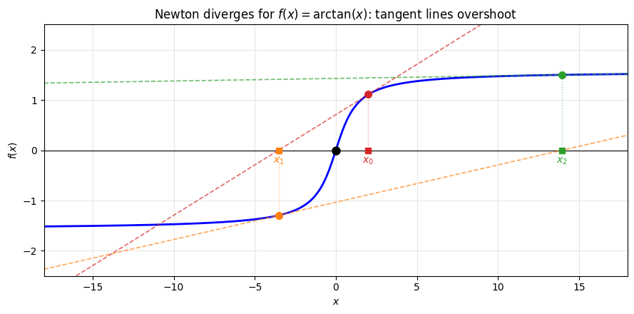

Newton iterates:
   k         x_k    |f(x_k)|   |f/f'|(x_k)
   0      2.0000    1.11e+00      5.54e+00
   1     -3.5357    1.30e+00      1.75e+01
   2     13.9510    1.50e+00      2.93e+02
   3   -279.3441    1.57e+00      1.22e+05

The iterates diverge: |x_k| grows at each step.
The residual |f(x_k)| also grows (though bounded by pi/2 for arctan).
The Newton correction |f/f'| grows even faster, reflecting the true error.

Quantitative Convergence: The Newton-Kantorovich Theorem¶

The local convergence theorem guarantees convergence if $\mathbf{x}_0$ is “close enough” to $\mathbf{x}^*$ . But how close is close enough? The Newton-Kantorovich theorem answers this using only information available at the initial point.

Theorem 1 (Newton-Kantorovich Theorem)

Let $\mathbf{F}$ be continuously differentiable with:

$D\mathbf{F}(\mathbf{x}_0)$ nonsingular with $\|[D\mathbf{F}(\mathbf{x}_0)]^{-1}\| \leq \beta$
$\|[D\mathbf{F}(\mathbf{x}_0)]^{-1}\mathbf{F}(\mathbf{x}_0)\| \leq \eta$ (size of first Newton step)
$\|D\mathbf{F}(\mathbf{x}) - D\mathbf{F}(\mathbf{y})\| \leq L\|\mathbf{x} - \mathbf{y}\|$ (Lipschitz constant)

If $h = \beta\eta L \leq \frac{1}{2}$ , then Newton’s method converges to a root $\mathbf{x}^*$ with:

\|\mathbf{x}^* - \mathbf{x}_0\| \leq \frac{1 - \sqrt{1 - 2h}}{h}\eta

(1)

The condition $h \leq 1/2$ combines three quantities:

How small the initial step is ( $\eta$ )
How sensitive the Jacobian is to changes ( $L$ )
How large the Jacobian inverse is ( $\beta$ )

Small $h$ means we’re in the “safe zone” for convergence. All three quantities can be computed (or bounded) at the starting point, without knowing the root.

The Kantorovich theorem tells us when convergence is guaranteed. When the conditions are not satisfied, we need strategies to make the method converge from farther away.

The fix is visible in the plot above: the tangent line is a good local approximation, but the full step overshoots because $\arctan$ flattens out far from the root. If we had taken only a fraction of the Newton step, the iterate would have moved toward zero instead of away from it. This motivates damped Newton: instead of taking the full step $\Delta\mathbf{x}$ , take a fraction:

\mathbf{x}_{k+1} = \mathbf{x}_k + \lambda_k \Delta\mathbf{x}_k

(2)

where $\lambda_k \in (0, 1]$ is the damping factor. The question is how to choose $\lambda_k$ , and this is where the two approaches diverge.

Approach 1: Backtracking Line Search¶

The simplest strategy: define a merit function that measures progress, and require each step to decrease it.

For root-finding, the natural merit function is the squared residual:

\phi(\mathbf{x}) = \frac{1}{2}\|\mathbf{F}(\mathbf{x})\|_2^2

(3)

Recall from the error analysis that the residual $\|\mathbf{F}(\hat{\mathbf{x}})\|$ is the backward error: it measures how well $\hat{\mathbf{x}}$ satisfies the equation. So backtracking on $\phi$ amounts to requiring each step to reduce the backward error.

The gradient of $\phi$ is $\nabla\phi(\mathbf{x}) = D\mathbf{F}(\mathbf{x})^T\mathbf{F}(\mathbf{x})$ , connecting root-finding to optimization.

The Armijo Condition¶

Start with $\lambda = 1$ (full Newton step) and reduce until we see sufficient decrease in $\phi$ .

Definition 1 (The Armijo Condition)

Accept step size $\lambda$ if:

\phi(\mathbf{x}_k + \lambda\Delta\mathbf{x}) \leq \phi(\mathbf{x}_k) + c\lambda \nabla\phi(\mathbf{x}_k)^T\Delta\mathbf{x}

(4)

where $c \in (0, 1)$ is a small constant (typically $c = 10^{-4}$ ).

The right-hand side is a linear prediction of $\phi$ along the search direction, scaled by $c$ . Since the Newton direction is a descent direction ( $\nabla\phi^T\Delta\mathbf{x} < 0$ when $D\mathbf{F}$ is nonsingular), this line has negative slope. The small $c$ makes the condition easy to satisfy: we just need some decrease, not optimal decrease.

Algorithm 1 (Backtracking Line Search)

Input: Current point $\mathbf{x}_k$ , Newton direction $\Delta\mathbf{x}$ , parameters $c \in (0, 1)$ , $\rho \in (0, 1)$

Output: Step size $\lambda$

$\lambda \gets 1$
while $\phi(\mathbf{x}_k + \lambda\Delta\mathbf{x}) > \phi(\mathbf{x}_k) + c\lambda \nabla\phi(\mathbf{x}_k)^T\Delta\mathbf{x}$ :
$\qquad \lambda \gets \rho \lambda$ (reduce step size)
return $\lambda$

Typical values: $c = 10^{-4}$ , $\rho = 0.5$ .

Properties¶

Far from solution: $\lambda_k$ is small, preventing overshoot.
Near solution: $\lambda_k = 1$ (full step accepted), recovering quadratic convergence.
Guaranteed progress: each iteration decreases $\phi$ .

Theorem 2 (Convergence of Backtracking Newton)

Under mild conditions on $\mathbf{F}$ , damped Newton with Armijo backtracking satisfies:

\lim_{k \to \infty} \|\nabla\phi(\mathbf{x}_k)\| = 0

(5)

If additionally the Jacobian is nonsingular at limit points, the method converges to a root.

Proof 1

Remark 1 (What “Global Convergence” Actually Means)

From Armijo to NLEQ-RES¶

The simple Armijo backtracking above halves $\lambda$ blindly until sufficient decrease is achieved. Deuflhard’s NLEQ-RES refines this with the same adaptive prediction machinery used by NLEQ-ERR (described below), but applied to the residual. The prediction uses a quadratic model along the Newton direction:

\mu_k = \frac{\frac{1}{2}\|\mathbf{F}(\mathbf{x}_k)\|\lambda_k^2}{\|\mathbf{F}(\mathbf{x}^{\text{trial}}) - (1 - \lambda_k)\mathbf{F}(\mathbf{x}_k)\|}

(6)

The reduced damping factor is $\lambda_k \gets \min(\mu_k, \lambda_k / 2)$ , and the monotonicity test can be either standard ( $\theta < 1$ ) or restricted ( $\theta < 1 - \lambda/4$ ). This gives NLEQ-RES faster convergence than naive backtracking while still monitoring the residual.

Limitations¶

Despite these improvements, damping based on $\|\mathbf{F}\|$ has a subtle flaw: it is not affine invariant. To understand why this matters, we first need to define what affine invariance means.

Affine Invariance¶

Definition 2 (Affine Invariance)

An iterative method for solving $\mathbf{F}(\mathbf{x}) = \mathbf{0}$ is affine invariant if it produces the same iterates (up to coordinate change) when applied to the transformed problem $\tilde{\mathbf{F}}(\mathbf{x}) = A\mathbf{F}(\mathbf{x})$ for any nonsingular matrix $A$ .

Why should we care? The matrix $A$ represents an arbitrary scaling or rotation of the equations. If we multiply the first equation by 1000, the mathematical problem is the same, but a non-invariant method may behave completely differently. An affine invariant method is insensitive to such choices.

Remark 2 (Newton’s Method is Affine Invariant)

Pure Newton’s method (with $\lambda = 1$ ) is affine invariant. Under $\tilde{\mathbf{F}} = A\mathbf{F}$ :

D\tilde{\mathbf{F}}^{-1}\tilde{\mathbf{F}} = (AD\mathbf{F})^{-1}(A\mathbf{F}) = D\mathbf{F}^{-1}\mathbf{F}

(7)

The Newton correction $\Delta\mathbf{x} = -D\mathbf{F}^{-1}\mathbf{F}$ is unchanged. But the residual norm $\|\tilde{\mathbf{F}}\| = \|A\mathbf{F}\| \neq \|\mathbf{F}\|$ in general.

So Newton itself is affine invariant, but Armijo backtracking on $\|\mathbf{F}\|$ breaks this invariance.

Approach 2: Error-Oriented Step Control (NLEQ-ERR)¶

Deuflhard’s insight: instead of monitoring the residual $\|\mathbf{F}\|$ (backward error), monitor the Newton correction $\|\Delta\mathbf{x}\|$ (forward error estimate). Since the Newton correction is affine invariant, this preserves the invariance of the overall method.

The Natural Level Function¶

The natural level function for error-oriented Newton is:

h(\mathbf{x}) = \|D\mathbf{F}(\mathbf{x})^{-1}\mathbf{F}(\mathbf{x})\| = \|\Delta\mathbf{x}\|

(8)

To see why this estimates the forward error, note that by the mean value theorem:

\mathbf{F}(\mathbf{x}) = \mathbf{F}(\mathbf{x}) - \mathbf{F}(\mathbf{x}^*) = D\mathbf{F}(\xi)(\mathbf{x} - \mathbf{x}^*)

(9)

for some $\xi$ between $\mathbf{x}$ and $\mathbf{x}^*$ . Inverting gives:

\mathbf{x} - \mathbf{x}^* = D\mathbf{F}(\xi)^{-1}\mathbf{F}(\mathbf{x}) \approx D\mathbf{F}(\mathbf{x})^{-1}\mathbf{F}(\mathbf{x}) = -\Delta\mathbf{x}

(10)

So the Newton correction is literally the linearized estimate of the error $\mathbf{x} - \mathbf{x}^*$ , and this estimate improves as $\mathbf{x} \to \mathbf{x}^*$ . This is the same principle as the step size lemma from the scalar case: if the iteration is contractive with factor $\theta < 1$ , then $\|\mathbf{x}_k - \mathbf{x}^*\| \leq \|\Delta\mathbf{x}_k\|/(1-\theta)$ . The contraction factor $\theta_k$ below plays exactly this role.

Monitoring $\|\Delta\mathbf{x}\|$ is the right choice because:

It estimates what we actually care about (distance to the root).
It is affine invariant ( $A$ cancels in $D\mathbf{F}^{-1}\mathbf{F}$ ).
Near the root, $\|\Delta\mathbf{x}\| \to 0$ is exactly the convergence criterion.

The Contraction Factor¶

After a damped step $\mathbf{x}_{k+1} = \mathbf{x}_k + \lambda_k\Delta\mathbf{x}_k$ with $\lambda_k \in (0, 1]$ , compute the simplified Newton correction at the trial point using the old Jacobian:

\overline{\Delta\mathbf{x}}_{k+1} = -D\mathbf{F}(\mathbf{x}_k)^{-1}\mathbf{F}(\mathbf{x}_{k+1})

(11)

The contraction factor is:

\theta_k = \frac{\|\overline{\Delta\mathbf{x}}_{k+1}\|}{\|\Delta\mathbf{x}_k\|}

(12)

This measures how much the error estimate shrank in one step. From the Banach fixed point theorem, convergence requires $\theta_k < 1$ (the iteration must be a contraction). Deuflhard uses a restricted monotonicity test:

\theta_k < 1 - \frac{\lambda_k}{4}

(13)

which is stronger than $\theta_k < 1$ and ensures well-controlled convergence.

Adaptive Step Size Prediction¶

A key feature of NLEQ_ERR: predict the optimal $\lambda$ rather than just halving when the test fails.

Two predictions are used. Within the damping loop (when a trial step is rejected), the prediction is based on the deviation between the actual and predicted corrections:

\mu_k^{\text{damp}} = \frac{\frac{1}{2}\|\Delta\mathbf{x}_k\|\lambda_k^2}{\|\overline{\Delta\mathbf{x}}_{k+1} - (1 - \lambda_k)\Delta\mathbf{x}_k\|}

(14)

The reduced damping factor is $\lambda_k \gets \min(\mu_k^{\text{damp}}, \lambda_k / 2)$ .

Between iterations (once a step is accepted), the prediction for the next iteration uses the ratio of successive corrections:

\mu_k^{\text{next}} = \frac{\|\Delta\mathbf{x}_{k-1}\| \cdot \|\overline{\Delta\mathbf{x}}_k\|}{\|\overline{\Delta\mathbf{x}}_k - \Delta\mathbf{x}_k\| \cdot \|\Delta\mathbf{x}_k\|} \cdot \lambda_k

(15)

The next damping factor is $\lambda_{k+1} = \min(1, \mu_k^{\text{next}})$ . Both predictions adapt aggressively: when the linearization is accurate ( $\mu$ is large), $\lambda$ ramps up quickly toward 1. When it is poor, $\lambda$ stays small.

An additional safeguard: if the predicted $\lambda$ would increase by a factor of 4 or more and no reduction occurred in the damping loop, the algorithm retries with the larger $\lambda$ before accepting the current step. This avoids accepting an overly conservative step when the prediction says a much larger step would succeed.

The Algorithm¶

Algorithm 2 (NLEQ_ERR (Simplified))

Input: $\mathbf{F}$ , $D\mathbf{F}$ , initial guess $\mathbf{x}_0$ , tolerance $\varepsilon$

Output: Approximate root $\mathbf{x}$

Choose initial $\lambda_0 \in (0, 1]$ (based on nonlinearity estimate: $\lambda_0 = 1$ for mildly nonlinear, $\lambda_0 = 10^{-2}$ for highly nonlinear, $\lambda_0 = 10^{-4}$ for extremely nonlinear)
for $k = 0, 1, 2, \ldots$ :
$\qquad$ Solve $D\mathbf{F}(\mathbf{x}_k)\Delta\mathbf{x}_k = -\mathbf{F}(\mathbf{x}_k)$
$\qquad$ if $\|\Delta\mathbf{x}_k\| < \varepsilon$ : return $\mathbf{x}_k + \Delta\mathbf{x}_k$
$\qquad$ Damping loop:
$\qquad\qquad$ $\mathbf{x}^{\text{trial}} \gets \mathbf{x}_k + \lambda_k\Delta\mathbf{x}_k$
$\qquad\qquad$ Solve $D\mathbf{F}(\mathbf{x}_k)\overline{\Delta\mathbf{x}} = -\mathbf{F}(\mathbf{x}^{\text{trial}})$ (reuse Jacobian)
$\qquad\qquad$ Compute $\theta_k = \|\overline{\Delta\mathbf{x}}\|/\|\Delta\mathbf{x}_k\|$
$\qquad\qquad$ if $\theta_k < 1 - \lambda_k/4$ : accept step, predict $\lambda_{k+1}$ from $\mu_k$
$\qquad\qquad$ else: $\lambda_k \gets \min(\mu_k, \lambda_k/2)$ , repeat damping loop
$\qquad$ $\mathbf{x}_{k+1} \gets \mathbf{x}^{\text{trial}}$

Note that step 7 reuses the Jacobian from step 3. The factored Jacobian is already available, so computing $\overline{\Delta\mathbf{x}}$ requires only a forward/backward substitution (cheap compared to a new factorization).

Theorem 3 (Local Quadratic Convergence Recovery)

For both methods: if $\mathbf{x}_k \to \mathbf{x}^*$ where $\mathbf{F}(\mathbf{x}^*) = \mathbf{0}$ and $D\mathbf{F}(\mathbf{x}^*)$ is nonsingular, then $\lambda_k = 1$ for all $k$ sufficiently large. Quadratic convergence is recovered near the root.

Proof 2

Visualization: Newton Fractals¶

The difference between these approaches is dramatically visible in the complex plane. Applying Newton’s method to $f(z) = z^3 - 1$ from a grid of starting points and coloring by which root the iteration converges to produces the classic Newton fractal. Backtracking on $|f(z)|$ does not eliminate the fractal (because $|f|$ has multiple valleys), while NLEQ-ERR’s error-oriented monitoring significantly smooths the basin boundaries.

Iteration Trajectories¶

The following example shows the iteration paths for all three methods applied to $f(z) = z^3 - 1$ from $z_0 = 0.35 + 0.22i$ , a starting point near a basin boundary where pure Newton bounces erratically before recovering. The left panel shows the trajectories in the complex plane overlaid on the Newton correction landscape $|f(z)/f'(z)|$ . The right panel compares the convergence histories.

import numpy as np
import matplotlib.pyplot as plt

f  = lambda z: z**3 - 1
df = lambda z: 3 * z**2
roots = np.array([np.exp(2j * np.pi * k / 3) for k in range(3)])

def newton_trajectory(f, df, z0, max_iter=50, tol=1e-12):
    """Pure Newton: full step every time."""
    path = [z0]
    z = z0
    for _ in range(max_iter):
        dfz = df(z)
        if abs(dfz) < 1e-15:
            break
        dz = f(z) / dfz
        z = z - dz
        path.append(z)
        if abs(dz) < tol:
            break
    return np.array(path)

def backtracking_trajectory(f, df, z0, max_iter=100, tol=1e-12):
    """Armijo backtracking: halve lambda until |f| decreases."""
    path = [z0]
    z = z0
    for _ in range(max_iter):
        fz = f(z)
        dfz = df(z)
        if abs(dfz) < 1e-15:
            break
        dz = fz / dfz
        lam = 1.0
        for _ in range(30):
            z_trial = z - lam * dz
            if abs(f(z_trial)) < abs(fz):
                break
            lam *= 0.5
        z = z_trial
        path.append(z)
        if abs(lam * dz) < tol:
            break
    return np.array(path)

def nleq_res_trajectory(f, df, z0, max_iter=100, tol=1e-12,
                        lambda_min=1e-4, restricted=True):
    """NLEQ-RES: Deuflhard's residual-based damped Newton."""
    path = [z0]
    z = z0
    normfk = abs(f(z))
    lam = 1.0
    mu = 1.0
    for k in range(max_iter):
        if normfk <= tol:
            break
        dfz = df(z)
        if abs(dfz) < 1e-15:
            break
        fz = f(z)
        dz = fz / dfz
        normdx = abs(dz)
        if k > 0:
            mu = (normfkm1 / normfk) * mu
            lam = min(1.0, mu)
        # Damping loop
        for _ in range(30):
            if lam < lambda_min:
                break
            z_trial = z + lam * dz  # dz = f/f', so step is x + lam*(f/f')
            # Wait — Newton step is x - f/f', so:
            z_trial = z - lam * dz
            fz_trial = f(z_trial)
            normfkp1 = abs(fz_trial)
            theta = normfkp1 / normfk
            # Prediction: mu = 0.5 * ||f_k|| * lam^2 / ||f_{k+1} - (1-lam)*f_k||
            w = fz_trial - (1 - lam) * fz
            mu = 0.5 * normfk * lam**2 / abs(w) if abs(w) > 1e-30 else 2.0 * lam
            # Monotonicity test
            if restricted:
                accept = theta < 1.0 - lam / 4.0
            else:
                accept = theta < 1.0
            if accept:
                break
            lam_new = min(mu, 0.5 * lam)
            lam = max(lam_new, lambda_min)
        z = z_trial
        path.append(z)
        normfkm1 = normfk
        normfk = normfkp1
        lam = min(1.0, mu)
        if normdx < tol:
            break
    return np.array(path)

def nleq_err_trajectory(f, df, z0, max_iter=100, tol=1e-12, lambda_min=1e-8):
    """NLEQ-ERR: error-oriented damped Newton (Deuflhard)."""
    path = [z0]
    z = z0
    # Adaptive initial lambda
    dz0 = f(z) / df(z)
    lam = min(1.0, 1.0 / abs(dz0)) if abs(dz0) > 1 else 1.0
    normdx_prev = abs(dz0)

    for _ in range(max_iter):
        dfz = df(z)
        if abs(dfz) < 1e-15:
            break
        dz = f(z) / dfz
        norm_dx = abs(dz)
        if norm_dx < tol:
            path.append(z - dz)
            break

        # Damping loop
        lam_trial = lam
        accepted = False
        for _ in range(30):
            z_trial = z - lam_trial * dz
            # Simplified Newton correction (reuse f'(z_k))
            dzbar = f(z_trial) / dfz
            normdxbar = abs(dzbar)
            theta = normdxbar / norm_dx if norm_dx > 1e-30 else 1.0

            if theta < 1.0 - lam_trial / 4.0:
                # Accept. Predict next lambda.
                w = abs(dzbar - (1 - lam_trial) * dz)
                if w > 1e-30:
                    mu = 0.5 * norm_dx * lam_trial**2 / w
                else:
                    mu = 2.0 * lam_trial
                lam = min(1.0, mu)
                accepted = True
                break
            else:
                # Reject. Reduce lambda.
                w = abs(dzbar - (1 - lam_trial) * dz)
                if w > 1e-30:
                    mu = 0.5 * norm_dx * lam_trial**2 / w
                else:
                    mu = 0.5 * lam_trial
                lam_trial = max(min(mu, 0.5 * lam_trial), lambda_min)
                if lam_trial <= lambda_min * 1.1:
                    accepted = True  # force accept with minimum lambda
                    break

        z = z - lam_trial * dz
        path.append(z)

        # Update lambda prediction from successive corrections
        if norm_dx > 1e-30 and normdx_prev > 1e-30:
            lam = min(1.0, normdx_prev * lam / norm_dx)
        lam = max(lam, lambda_min)
        normdx_prev = norm_dx

    return np.array(path)

z0 = 0.354 + 0.219j

path_newton = newton_trajectory(f, df, z0, max_iter=30)
path_bt     = backtracking_trajectory(f, df, z0)
path_res    = nleq_res_trajectory(f, df, z0)
path_err    = nleq_err_trajectory(f, df, z0)

fig = plt.figure(figsize=(10, 12), layout='constrained')
gs = fig.add_gridspec(2, 4, height_ratios=[2.5, 1])

# --- Top: trajectories in the complex plane (spans all 4 columns) ---
ax_top = fig.add_subplot(gs[0, :])

N = 400
x = np.linspace(-2, 2, N)
y = np.linspace(-2, 2, N)
xx, yy = np.meshgrid(x, y)
zz = xx + 1j * yy
dfzz = df(zz)
safe = np.abs(dfzz) > 1e-15

# Newton correction landscape: |f/f'|
correction = np.full_like(xx, np.nan)
correction[safe] = np.log10(np.abs(f(zz[safe]) / dfzz[safe]) + 1e-16)

im = ax_top.pcolormesh(xx, yy, correction, shading='auto', vmin=-2, vmax=1,
                       cmap='viridis')
plt.colorbar(im, ax=ax_top, label=r"$\log_{10}|f/f'|$",
             orientation='horizontal', fraction=0.05, pad=0.08)

for path, color, label, marker in [
    (path_newton, '#d62728', 'Newton', 'o'),
    (path_bt,     '#ff7f0e', 'Backtracking', '^'),
    (path_res,    'black', 'NLEQ-RES', 's'),
    (path_err,    '#1f77b4', 'NLEQ-ERR', 'D')]:
    ax_top.plot(path.real, path.imag, '-', color=color, linewidth=3, alpha=0.9)
    ax_top.plot(path.real, path.imag, marker, color=color, markersize=5,
                zorder=4, markeredgecolor='white', markeredgewidth=0.5)
    ax_top.plot(path[0].real, path[0].imag, '*', color='#2ca02c',
                markersize=16, zorder=5, markeredgecolor='black',
                markeredgewidth=1)
    ax_top.plot(path[-1].real, path[-1].imag, marker, color=color,
                markersize=7, zorder=5, label=label)

ax_top.scatter(roots.real, roots.imag, c='white', s=120, zorder=6,
               edgecolors='black', linewidths=2, marker='*')
ax_top.set_xlabel('Re($z$)', fontsize=12)
ax_top.set_ylabel('Im($z$)', fontsize=12)
ax_top.set_title(r"Iteration trajectories on the $|f/f'|$ landscape")
ax_top.set_aspect('equal')
ax_top.legend(fontsize=9, loc='lower left')
ax_top.set_xlim(-2, 2)
ax_top.set_ylim(-2, 2)

# --- Bottom left: residual |f(z_k)| (narrower than top) ---
ax_res = fig.add_subplot(gs[1, 0:2])

for path, color, label in [
    (path_newton, '#d62728', 'Newton'),
    (path_bt,     '#ff7f0e', 'Backtracking'),
    (path_res,    'black', 'NLEQ-RES'),
    (path_err,    '#1f77b4', 'NLEQ-ERR')]:
    residuals = np.abs(f(path))
    n = np.arange(len(path))
    ax_res.semilogy(n, residuals, '-o', color=color, markersize=4,
                    linewidth=2, label=label)

ax_res.set_xlabel('Iteration $k$', fontsize=11)
ax_res.set_ylabel(r'$|f(z_k)|$', fontsize=11)
ax_res.set_title('Residual (backward error)')
ax_res.legend(fontsize=8)
ax_res.grid(True, alpha=0.3, which='both')
ax_res.set_xlim(left=0)
ax_res.set_ylim(bottom=1e-16)

# --- Bottom right: Newton correction |f/f'| (forward error estimate) ---
ax_err = fig.add_subplot(gs[1, 2:4])


for path, color, label in [
    (path_newton, '#d62728', 'Newton'),
    (path_bt,     '#ff7f0e', 'Backtracking'),
    (path_res,    'black', 'NLEQ-RES'),
    (path_err,    '#1f77b4', 'NLEQ-ERR')]:
    dfpath = df(path)
    safe_p = np.abs(dfpath) > 1e-15
    corrections = np.full(len(path), np.nan)
    corrections[safe_p] = np.abs(f(path[safe_p]) / dfpath[safe_p])
    n = np.arange(len(path))
    ax_err.semilogy(n, corrections, '-o', color=color, markersize=4,
                    linewidth=2, label=label)

ax_err.set_xlabel('Iteration $k$', fontsize=11)
ax_err.set_ylabel(r"$|f(z_k)/f'(z_k)|$", fontsize=11)
ax_err.set_title('Newton correction (forward error estimate)')
ax_err.legend(fontsize=8)
ax_err.grid(True, alpha=0.3, which='both')
ax_err.set_xlim(left=0)
ax_err.set_ylim(bottom=1e-16)

plt.show()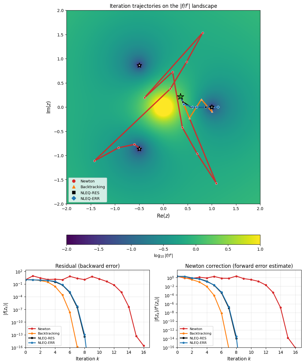

Iteration trajectories for $f(z) = z^3 - 1$ from $z_0 = 0.35 + 0.22i$ . Top: Paths in the complex plane overlaid on the Newton correction landscape $|f/f'|$ (darker = closer to a root). Pure Newton (red) bounces between all three basins before settling. Simple Armijo backtracking (orange) damps by halving $\lambda$ until $|f|$ decreases. NLEQ-RES (black) uses Deuflhard’s residual-based damping with predicted step sizes. NLEQ-ERR (blue) damps based on the correction norm. Bottom left: The residual $|f(z_k)|$ (backward error). Bottom right: The Newton correction $|f(z_k)/f'(z_k)|$ (forward error estimate, matching the landscape above). The damped methods converge monotonically while undamped Newton oscillates.

Reference: P. Deuflhard, Newton Methods for Nonlinear Problems: Affine Invariance and Adaptive Algorithms, Springer, 2011.