Differentiation as a Matrix

Two Pictures of Differentiation¶

We have already met the local picture: forward differences give $O(h)$ accuracy and centered differences give $O(h^2)$. Each derivative estimate uses 2–3 nearby values; the rest of the data is ignored.

The spectral picture is the opposite. The interpolant $p_n$ already encodes all the data globally. Its derivative $p_n'$ is just another polynomial in $\mathbb{P}_{n-1} \subset \mathbb{P}_n$, which we can in turn represent by its values at the same Chebyshev nodes or by its Chebyshev coefficients. So differentiation is a linear map from $\mathbb{P}_n$ to itself, and the question is: what does its matrix look like in each of the two bases?

A naming convention before we start. Throughout this section and the next we use “coefficient space” and “value space” as shorthand for two specific bases of $\mathbb{P}_n$:

• Coefficient space is the Chebyshev basis $\{T_k\}$. The coordinates are the Chebyshev coefficients $(c_0, \ldots, c_n)$.

• Value space is the Lagrange basis $\{\ell_j\}$. The coordinates of a polynomial in this basis are literally its nodal values $(f_0, \ldots, f_n)$, since $p_n(x) = \sum_j f_j\, \ell_j(x)$.

Both are bases of the same $(n+1)$-dimensional space $\mathbb{P}_n$. The DCT from §2 is precisely the change-of-basis matrix between them. The “coefficient-space” operator $\mathcal{D}$ below represents differentiation in the Chebyshev basis; the “value-space differentiation matrix” $D$ represents the same map in the Lagrange basis.

Differentiation in the Coefficient Basis¶

In the Chebyshev (coefficient) basis the polynomial is

We want the coefficients $c'_k$ of $p_n'$ in the same basis:

The derivation begins with a single chain-rule calculation that, by itself, forces a new family of polynomials onto the stage.

Step 1: Differentiate $T_k$ by the chain rule¶

Recall that $T_k(x) = \cos(k\theta)$ where $x = \cos\theta$, so $\dfrac{d\theta}{dx} = -\dfrac{1}{\sin\theta}$. Differentiating,

The factor $\sin(k\theta)/\sin\theta$ looks transcendental but is in fact a polynomial in $x = \cos\theta$. The argument is short enough to spell out.

Start with the product-to-sum identity $\sin(A+B) - \sin(A-B) = 2\cos A \sin B$. Setting $A = \theta$, $B = (k-1)\theta$ and using $\sin(2-k)\theta = -\sin(k-2)\theta$,

Define $u_k(x) := \sin\!\big((k+1)\theta\big)/\sin\theta$. Dividing the identity above by $\sin\theta$ and reindexing turns it into a recurrence on $u_k$,

For the base cases,

The recurrence with these starting values produces a polynomial at every step: if $u_{k-1}$ and $u_{k-2}$ are polynomials of degrees $k-1$ and $k-2$, then $2x\,u_{k-1} - u_{k-2}$ is a polynomial of degree $k$. By induction $u_k$ is a polynomial of degree $k$. So $\sin(k\theta)/\sin\theta = u_{k-1}(x)$ is a polynomial of degree $k-1$ in $x$. Cranking the recurrence by hand,

Note that this is the same three-term recurrence as $T_k$, with the same first step $u_1 = 2x = 2 T_1$ but a different zeroth value ($u_0 = 1 = T_0$). So $u_k$ and $T_k$ are siblings: same growth recurrence, different boundary conditions.

Step 2: That polynomial has a name¶

The polynomial $u_k$ that just dropped out of the chain rule is what is conventionally called the Chebyshev polynomial of the second kind, written $U_k$:

With this name the chain-rule output is

That is the first identity.

Step 3: Express $T_j$ back in the $U$ basis¶

To finish the derivation we need to translate between the two bases. The product-to-sum formula for $\cos(j\theta)\sin\theta$ gives

i.e., a $T_j$ is the half-difference of two consecutive $U$’s.

Now differentiate $p_n = \sum_k c_k T_k$ term by term with the first identity,

On the other hand, writing $p_n' = \sum_j c'_j\, T_j$ and substituting the second identity in the form $T_j = \tfrac{1}{2}(U_j - U_{j-2})$,

The polynomial $p_n'$ has the same expansion in the $U$ basis under both forms, so the coefficients of each $U_j$ must match. Reindex the first sum by $k = m + 1$ so that $U_{k-1} = U_m$ contributes $(m+1)\, c_{m+1}$ to the coefficient of $U_m$. Matching,

Setting $k = m + 1$ gives the backward two-term recurrence stated below.

This is differentiation in the coefficient basis. In matrix terms, the operator is the strictly upper-triangular, banded matrix

with non-trivial entries only on every other super-diagonal.

Source

import numpy as np
import matplotlib.pyplot as plt
import scipy.fft as fft

def chebpts(N): return np.cos(np.pi * np.arange(N+1)/N)

def vals2coeffs(v):
    n = len(v) - 1
    c = fft.dct(v[::-1], type=1, norm='forward')
    c[1:n] *= 2
    return c

def coeffs2vals(c):
    n = len(c) - 1
    cs = c.copy(); cs[1:n] /= 2
    v = fft.idct(cs, type=1, norm='forward')
    return v[::-1]

def coeff_diff_matrix(N):
    """Banded operator that maps Chebyshev coefficients of p_n
    to Chebyshev coefficients of p_n' (length N+1, last entry zero)."""
    M = np.zeros((N+1, N+1))
    for k in range(N, 0, -1):
        # c'_{k-1} = c'_{k+1} + 2k c_k
        M[k-1, k] += 2*k
        if k+1 <= N:
            M[k-1, :] += M[k+1, :]
    M[0, :] /= 2
    return M

D_coeff = coeff_diff_matrix(16)
fig, ax = plt.subplots(figsize=(5.5, 5))
ax.spy(D_coeff, markersize=6)
ax.set_title(r'Coefficient-space $\mathcal{D}$ (banded), $N = 16$')
plt.tight_layout(); plt.show()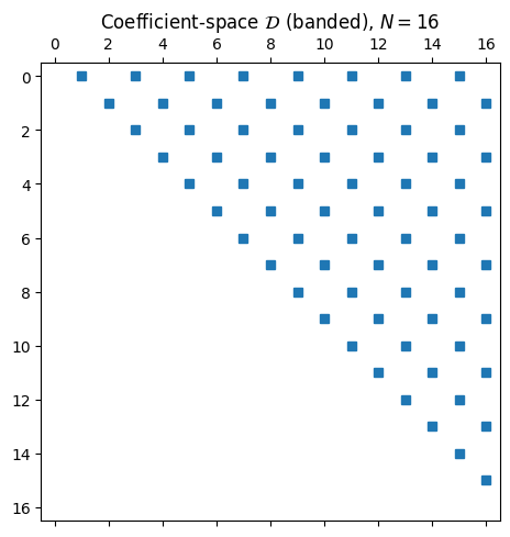

Applying $\mathcal{D}$ costs $O(N)$ because of the bandedness. The two DCTs that go from values to coefficients and back each cost $O(N \log N)$, so the whole values $\to$ derivative-values pipeline is $O(N \log N)$.

Differentiation in the Value Basis¶

In the Lagrange (value) basis the polynomial is

so

Evaluating $p_n'$ at the same nodes $x_i$ gives

This is a matrix-vector product. Define the value-space differentiation matrix $D \in \mathbb{R}^{(n+1)\times(n+1)}$ by

The entries of $D$ are determined entirely by the nodes, not by $f$. Compute them once and you can differentiate any function sampled on those nodes by a single matrix-vector multiplication.

Closed-form entries from the barycentric formula¶

Recall from §1 that the barycentric form of the Lagrange basis is

Differentiating $\ell_j$ by the product rule and evaluating at $x = x_i$ with $i \ne j$, the term containing $\ell(x_i) = 0$ drops out and one obtains, after some algebra,

The diagonal entries follow from a separate trick: since the constant function 1 is its own interpolant, $\sum_j \ell_j(x) \equiv 1$, so differentiating gives $\sum_j \ell_j'(x) \equiv 0$. Evaluated at $x = x_i$, this says the rows of $D$ sum to zero:

For Chebyshev nodes $x_j = \cos(j\pi/n)$ the barycentric weights are $\lambda_j = (-1)^j \delta_j$ with $\delta_0 = \delta_n = \tfrac12$ and $\delta_j = 1$ otherwise, so the formula evaluates without any extra work. The value-space matrix $D$ is dense: every output value $p_n'(x_i)$ depends on every input value $f_j$. That is the price of using a global interpolant.

Source

def cheb_diff_matrix(N):
    if N == 0:
        return np.zeros((1, 1)), np.zeros(1)
    x = np.cos(np.pi * np.arange(N+1) / N)
    c = np.ones(N+1); c[0] = 2; c[N] = 2; c[1::2] *= -1
    X = np.outer(x, np.ones(N+1))
    dX = X - X.T + np.eye(N+1)
    D = np.outer(c, 1/c) / dX
    D -= np.diag(D.sum(axis=1))
    return D, x

f  = lambda x: np.exp(np.sin(5*x))
fp = lambda x: 5*np.cos(5*x) * np.exp(np.sin(5*x))

fig, axes = plt.subplots(1, 2, figsize=(11, 4.4))

D, _ = cheb_diff_matrix(16)
im = axes[0].imshow(np.abs(D), cmap='viridis',
                    norm=plt.matplotlib.colors.LogNorm())
axes[0].set_title(r'Value-space matrix $|D|$, $N = 16$')
plt.colorbar(im, ax=axes[0], fraction=0.046)

Ns = np.arange(4, 81, 2)
err_spec, err_fd2 = [], []
for N in Ns:
    D, x = cheb_diff_matrix(N)
    err_spec.append(np.max(np.abs(D @ f(x) - fp(x))))
    xu = np.linspace(-1, 1, N+1); h = xu[1] - xu[0]
    fu = f(xu); df = np.empty_like(fu)
    df[1:-1] = (fu[2:] - fu[:-2]) / (2*h)
    df[0]  = (fu[1] - fu[0]) / h
    df[-1] = (fu[-1] - fu[-2]) / h
    err_fd2.append(np.max(np.abs(df - fp(xu))))

axes[1].semilogy(Ns, err_spec, 'o-', label='Chebyshev $D$')
axes[1].semilogy(Ns, err_fd2, 's-', label='2nd-order centred FD')
axes[1].set_xlabel('$N$'); axes[1].set_ylabel(r"$\|D \mathbf{f} - f'\|_\infty$")
axes[1].set_title(r"Convergence on $e^{\sin 5x}$")
axes[1].legend()
plt.tight_layout(); plt.show()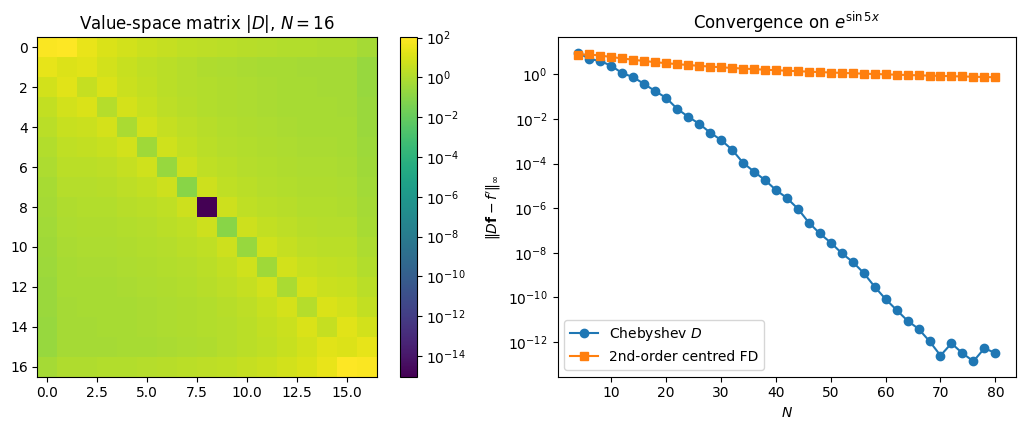

The left panel is the structure of $D$ at $N = 16$: every entry is nonzero, and the corner entries dominate (the $(0,0)$ and $(N,N)$ entries equal $\pm (2N^2 + 1)/6$). Those large boundary entries are exactly what allows boundary conditions to influence the interior in spectral BVP solvers (§7).

The right panel is convergence on $f(x) = e^{\sin 5x}$, an entire function. Centered differences drop algebraically as $N^{-2}$. Chebyshev differentiation drops geometrically: it reaches machine precision near $N \approx 30$ and stays there. By the regularity-decay dictionary, the differentiation error inherits the convergence rate of $p_n \to f$, with at most a single power of $N$ lost in differentiation. Same dictionary also predicts that on a non-smooth $f$ both schemes drop to algebraic and the spectral edge disappears.

Compare to the coefficient-space matrix above: the value-space matrix has every entry nonzero, so applying $D$ costs $O(N^2)$, while the coefficient-space pipeline costs $O(N \log N)$. Both bases produce the same derivative to within rounding error.

Source

N = 16
D_value, _ = cheb_diff_matrix(N)
D_coeff    = coeff_diff_matrix(N)

x = chebpts(N); v = f(x)
deriv_via_value = D_value @ v
c = vals2coeffs(v)
cprime = D_coeff @ c
deriv_via_coeff = coeffs2vals(cprime)

fig, axes = plt.subplots(1, 2, figsize=(11, 4.4))
axes[0].spy(D_value, markersize=6)
axes[0].set_title(r'Value-space $D$ (dense), $N = 16$')
axes[1].spy(D_coeff, markersize=6)
axes[1].set_title(r'Coefficient-space $\mathcal{D}$ (banded)')
plt.tight_layout(); plt.show()

err = np.max(np.abs(deriv_via_value - deriv_via_coeff))
print(f'max |D f - C^(-1) D_coeff C f|  =  {err:.2e}')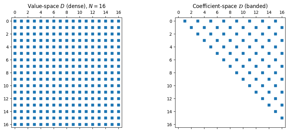

max |D f - C^(-1) D_coeff C f|  =  1.39e+01

Two basis choices, two completely different sparsity patterns, identical answer to within rounding error.

Choose the Basis That Makes the Operation Easy¶

The bigger point of this section is one we will keep returning to. Polynomial calculus offers us a choice of representation for every operation, and we are free to pick whichever is cheapest. Sampling a function and multiplying two polynomials pointwise are easy in the value basis. Reading off smoothness from coefficient decay, truncating to degree $n$, and integrating against the Chebyshev weight (as we saw in §4) are easy in the coefficient basis. Translating between the two costs a single DCT, that is $O(N \log N)$, so we move freely between them.

The same tension will reappear in later sections. Finding polynomial roots via an eigenvalue problem (§6) produces a sparse, well-conditioned matrix in the Chebyshev basis and an ill-conditioned one in the monomial basis. Spectral BVP solvers (§7) turn on exactly the same choice: value-space collocation gives a dense system, while a coefficient-space (ultraspherical) representation gives a banded one. In both cases, picking the right basis is what turns an intractable problem into a practical one.