Practical Root Finding - Introduction to Scientific Computing

Big Idea

Real-world problems often have multiple roots, and we need to find all of them reliably. This requires combining bracketing (to isolate roots) with fast solvers (to compute them accurately). Production solvers like MATLAB’s fzero and SciPy’s brentq use hybrid methods that get the best of both worlds.

The Challenge: Multiple Roots¶

So far we have studied methods that converge to one root:

Bisection is safe but slow, and requires a bracket $[a, b]$ with $f(a)f(b) < 0$ .
Newton’s method is fast but local: it converges to whichever root is nearest (roughly), and may miss others entirely.

In practice, a function can have many roots, and we need a systematic way to find them all.

Example 1 (Multiple Roots)

Consider $f(x) = x^3 - 6x^2 + 11x - 6 = (x-1)(x-2)(x-3)$ . There are three roots at $x = 1, 2, 3$ . Starting Newton’s method from $x_0 = 0$ converges to $x = 1$ . Starting from $x_0 = 2.5$ converges to $x = 3$ (not the nearest root $x = 2$ ). There is no single starting point that finds all three.

Bracketing¶

The first step is to isolate each root in its own interval. The simplest approach: evaluate $f$ on a grid and look for sign changes.

Algorithm 1 (Sign-Change Scanning)

Input: Function $f$ , interval $[a, b]$ , number of sample points $N$

Output: List of brackets $[a_i, b_i]$ with $f(a_i)f(b_i) < 0$

Set $h = (b - a)/N$
for $i = 0, 1, \ldots, N-1$ :
$\qquad$ $x_i = a + ih$ , $x_{i+1} = a + (i+1)h$
$\qquad$ if $f(x_i) \cdot f(x_{i+1}) < 0$ : record bracket $[x_i, x_{i+1}]$

By the Intermediate Value Theorem, each bracket contains at least one root.

Remark 1 (Limitations of Sign-Change Scanning)

This approach can miss roots in two situations:

Even-multiplicity roots (e.g., $f(x) = x^2$ ): the function touches zero but does not change sign, so no bracket is detected.
Closely spaced roots: if two roots are closer than the grid spacing $h$ , they may fall in the same interval. The sign change detects only one bracket, and bisection/Newton applied to that bracket may find only one of the two roots.

A finer grid reduces the chance of missing roots but increases the cost.

import numpy as np
import matplotlib.pyplot as plt

f = lambda x: x**3 - 6*x**2 + 11*x - 6

x = np.linspace(-0.5, 4, 500)
fig, ax = plt.subplots(figsize=(8, 4))
ax.plot(x, f(x), 'b-', linewidth=2)
ax.axhline(0, color='k', linewidth=0.8)

# Sign-change scanning
N = 20
x_grid = np.linspace(-0.5, 4, N + 1)
f_grid = f(x_grid)

brackets = []
for i in range(N):
    if f_grid[i] * f_grid[i + 1] < 0:
        brackets.append((x_grid[i], x_grid[i + 1]))
        ax.axvspan(x_grid[i], x_grid[i + 1], alpha=0.2, color='green')

# Mark roots
roots = [1, 2, 3]
for r in roots:
    ax.plot(r, 0, 'ro', markersize=8, zorder=5)

ax.set_xlabel('$x$')
ax.set_ylabel('$f(x)$')
ax.set_title(f'Sign-change scanning: {len(brackets)} brackets found (green)')
ax.grid(True, alpha=0.3)
ax.set_ylim(-3, 3)
plt.tight_layout()
plt.show()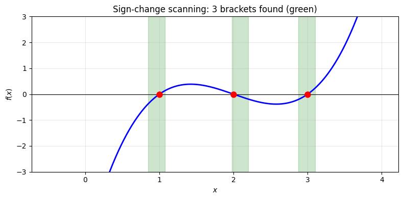

Finding All Roots¶

Once we have brackets, apply a fast solver to each one independently. This is the bracket-then-solve strategy.

Algorithm 2 (Find All Roots)

Input: Function $f$ , interval $[a, b]$ , grid size $N$ , tolerance $\varepsilon$

Output: List of all detected roots

Scan: evaluate $f$ on a grid of $N+1$ points in $[a, b]$ .
Bracket: identify all intervals $[x_i, x_{i+1}]$ where $f$ changes sign.
Solve: apply Brent’s method (or Newton-bisection) to each bracket.
Deduplicate: remove any roots that are within $\varepsilon$ of each other.

from scipy.optimize import brentq

def find_all_roots(f, a, b, N=1000, tol=1e-12):
    """Find all sign-change roots of f on [a, b]."""
    x_grid = np.linspace(a, b, N + 1)
    f_grid = f(x_grid)

    roots = []
    for i in range(N):
        if f_grid[i] * f_grid[i + 1] < 0:
            root = brentq(f, x_grid[i], x_grid[i + 1], xtol=tol)
            # Deduplicate
            if not roots or abs(root - roots[-1]) > 10 * tol:
                roots.append(root)
    return roots

# Example: find all roots of a more complex function
g = lambda x: np.sin(5*x) * np.exp(-x/3) - 0.1

roots_found = find_all_roots(g, 0, 10)

fig, ax = plt.subplots(figsize=(10, 4))
x = np.linspace(0, 10, 1000)
ax.plot(x, g(x), 'b-', linewidth=2)
ax.axhline(0, color='k', linewidth=0.8)
for r in roots_found:
    ax.plot(r, 0, 'ro', markersize=8, zorder=5)
ax.set_xlabel('$x$')
ax.set_ylabel('$f(x)$')
ax.set_title(f'Found {len(roots_found)} roots of $\\sin(5x) e^{{-x/3}} - 0.1$')
ax.grid(True, alpha=0.3)
plt.tight_layout()
plt.show()

print("Roots found:")
for i, r in enumerate(roots_found):
    print(f"  x_{i} = {r:.10f},  f(x_{i}) = {g(r):.2e}")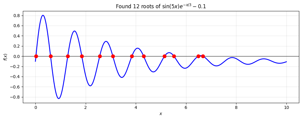

Roots found:
  x_0 = 0.0201690821,  f(x_0) = 0.00e+00
  x_1 = 0.6037981464,  f(x_1) = -1.25e-16
  x_2 = 1.2874784697,  f(x_2) = 3.92e-14
  x_3 = 1.8477141366,  f(x_3) = -5.55e-16
  x_4 = 2.5606764392,  f(x_4) = -3.19e-16
  x_5 = 3.0849105381,  f(x_5) = 6.59e-15
  x_6 = 3.8435849184,  f(x_6) = -1.49e-13
  x_7 = 4.3113522549,  f(x_7) = 4.36e-15
  x_8 = 5.1443525356,  f(x_8) = -1.80e-16
  x_9 = 5.5187146940,  f(x_9) = -5.80e-15
  x_10 = 6.4947954040,  f(x_10) = 6.25e-16
  x_11 = 6.6750973502,  f(x_11) = 2.78e-17

Hybrid Methods¶

No single method is perfect. Bisection is safe but slow. Newton is fast but can diverge. The most robust solvers combine both: maintain a bracket that always contains the root, but use faster steps when possible. Even these have limitations, as we will see.

Brent’s Method¶

Brent’s method (1973) combines three strategies:

Bisection: always safe, always shrinks the bracket by half.
Secant method: uses the two most recent points to extrapolate (no derivative needed, superlinear convergence).
Inverse quadratic interpolation: fits a parabola through the three most recent points for even faster convergence.

At each step, Brent’s method tries the fastest option first (inverse quadratic interpolation), falls back to secant if that fails, and uses bisection as the last resort. The bracket is always maintained, so convergence is guaranteed.

This is what MATLAB’s fzero and SciPy’s brentq implement. The difference is that fzero(f, x0) can search for a bracket starting from a single guess, while brentq(f, a, b) requires the bracket up front.

Newton-Bisection Hybrid¶

An alternative is to maintain a bracket and use Newton steps when they stay inside the bracket, falling back to bisection otherwise. This is sometimes called safe Newton. It requires the derivative $f'$ but converges quadratically near the root while still guaranteeing convergence globally.

Brent’s method avoids requiring the derivative, which makes it more broadly applicable.

Deflation¶

Instead of bracketing all roots up front, deflation finds roots one at a time. After finding a root $r_1$ , divide it out and solve the deflated problem.

For a polynomial $f(x)$ with a known root $r_1$ , define:

f_1(x) = \frac{f(x)}{x - r_1}

(1)

The roots of $f_1$ are the remaining roots of $f$ . Apply any solver to $f_1$ to find the next root, then deflate again.

Remark 2 (Practical Considerations for Deflation)

Systems of Equations¶

For systems $F(\mathbf{x}) = \mathbf{0}$ , bracketing no longer applies since there is no notion of sign change in multiple dimensions. The locality problem becomes much harder: Newton’s method still converges quadratically near a solution, but can diverge wildly from a poor initial guess.

Several techniques exist to make Newton’s method more robust for systems. Globalization strategies such as damped Newton and backtracking line searches restrict step sizes to prevent divergence. Quasi-Newton methods like Broyden’s method avoid computing the full Jacobian at every step, reducing cost from $\mathcal{O}(n^3)$ to $\mathcal{O}(n^2)$ per iteration. These ideas are developed in the Nonlinear Systems chapter.