Finite Difference Method

Finite Difference Method#

import numpy as np
import scipy.linalg as la
import matplotlib.pyplot as plt

Consider a second order linear differential equation with boundary conditions

y^{″} + p (t) y^{'} + q (t) y = r (t), y (t_{0}) = α, y (t_{f}) = β

The finite difference method is:

Discretize the domain: choose $N$ , let $h = (t_{f} - t_{0}) / (N + 1)$ and define $t_{k} = t_{0} + k h$ .
Let $y_{k} \approx y (t_{k})$ denote the approximation of the solution at $t_{k}$ .
Substitute finite difference formulas into the equation to define an equation at each $t_{k}$ .
Rearrange the system of equations into a linear system $A y = b$ and solve for $ $y = {[\begin{matrix} y_{1} & y_{2} & \dots & y_{N} \end{matrix}]}^{T}$ $

For example, consider an equation of the form

y^{″} = r (t), y (t_{0}) = α, y (t_{f}) = β

Choose $N$ , let $h = (t_{f} - t_{0}) / (N + 1)$ and Llet $r_{k} = r (t_{k})$ . The finite difference method yields the linear system $A y = b$ where

\begin{array}{r} A = [\begin{array}{rrcrr} - 2 & 1 \\ 1 & - 2 & 1 \\ ⋱ \\ 1 & - 2 & 1 \\ 1 & - 2 \end{array}] b = [\begin{array}{c} h^{2} r_{1} - α \\ h^{2} r_{2} \\ ⋮ \\ h^{2} r_{N - 1} \\ h^{2} r_{N} - β \end{array}] \end{array}

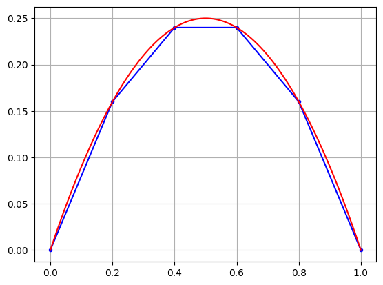
Example 1#

Plot the approximation for the equation

y^{″} = - 2, y (0) = 0, y (1) = 0

and compare to the exact solution

y (t) = t - t^{2}

t0 = 0; tf = 1; alpha = 0; beta = 0;
N = 4; h = (tf - t0)/(N + 1)

t = np.linspace(t0,tf,N+2)
r = -2*np.ones(t.size)

A = np.diag(np.repeat(-2,N)) + np.diag(np.repeat(1,N-1),1) + np.diag(np.repeat(1,N-1),-1)
b = h**2*r[1:N+1] - np.concatenate([alpha,np.zeros(N-2),beta],axis=None)
y = la.solve(A,b)

y = np.concatenate([alpha,y,beta],axis=None)
plt.plot(t,y,'b.-')

T = np.linspace(t0,tf,100)
Y = T*(1 - T)
plt.plot(T,Y,'r')
plt.grid(True)
plt.show()

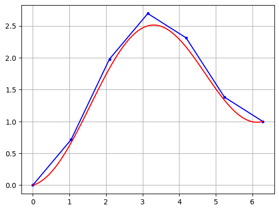
../_images/3dcf03d858448052a01a6edeebd6ee8d0d4ac84ca8dfc905ec78bd9ae049bc08.png

Example 2#

Plot the approximation for the equation

y^{″} = \cos (t), y (0) = 0, y (2 π) = 1

and compare to the exact solution

y (t) = 1 - \cos (t) + \frac{t}{2 π}

t0 = 0; tf = 2*np.pi; alpha = 0; beta = 1;
N = 5; h = (tf - t0)/(N + 1);

t = np.linspace(t0,tf,N+2)
r = np.cos(t)

A = np.diag(np.repeat(-2,N)) + np.diag(np.repeat(1,N-1),1) + np.diag(np.repeat(1,N-1),-1)
b = h**2*r[1:N+1] - np.concatenate([alpha,np.zeros(N-2),beta],axis=None)
y = la.solve(A,b)

y = np.concatenate([alpha,y,beta],axis=None)
plt.plot(t,y,'b.-')

T = np.linspace(t0,tf,100)
Y = 1-np.cos(T) + T/2/np.pi
plt.plot(T,Y,'r')
plt.grid(True)
plt.show()

../_images/c25bd78c862bdb0d63f8aa8326a35b381adf1c84b6769ded5b3c265e1df39f1c.png

Example 3#

Consider a general second order linear ordinary differential equation with boundary conditions

y^{″} + p (t) y^{'} + q (t) y = r (t), y (t_{0}) = α, y (t_{f}) = β

Introduce the notation

a_{k} = 1 - \frac{h p_{k}}{2} b_{k} = h^{2} q_{k} - 2 c_{k} = 1 + \frac{h p_{k}}{2}

The finite difference method yields the linear system $A y = b$ where

\begin{array}{r} A = [\begin{array}{rrcrr} b_{1} & c_{1} \\ a_{2} & b_{2} & c_{2} \\ ⋱ \\ a_{N - 1} & b_{N - 1} & c_{N - 1} \\ a_{N} & b_{N} \end{array}] b = [\begin{array}{c} h^{2} r_{1} - (1 - h p_{1} / 2) α \\ h^{2} r_{2} \\ ⋮ \\ h^{2} r_{N - 1} \\ h^{2} r_{N} - (1 + h p_{N} / 2) β \end{array}] \end{array}

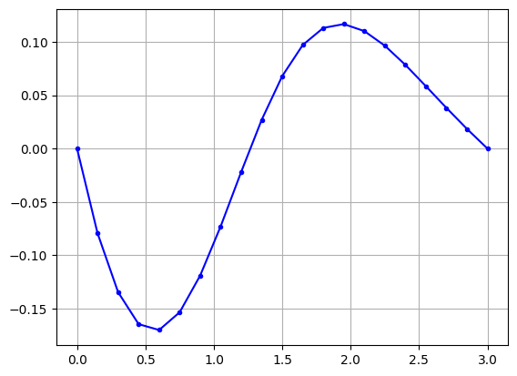
Plot the approximation for the equation

y^{″} + t^{2} y^{'} + y = \cos (t), y (0) = 0, y (3) = 0

alpha = 0; beta = 0; N = 19;
t0 = 0; tf = 3; h = (tf - t0)/(N + 1);
t = np.linspace(t0,tf,N+2)

p = t**2
q = np.ones(t.size)
r = np.cos(t)

a = 1 - h*p/2
b = h**2*q - 2
c = 1 + h*p/2
A = np.diag(b[1:N+1]) + np.diag(c[1:N],1) + np.diag(a[2:N+1],-1)

b = h**2*r[1:N+1] - np.concatenate([a[1]*alpha,np.zeros(N-2),c[N]*beta],axis=None)
y = la.solve(A,b)

y = np.concatenate([alpha,y,beta],axis=None)
plt.plot(t,y,'b.-')
plt.grid(True)
plt.show()

../_images/8f80301c48aa26eb5ece751e45555cc8c7fb16eb957a8ebdc7c28cf90806ee86.png

Finite Difference Method

Contents

Finite Difference Method#

Example 1#

Example 2#

Example 3#