Spectral Methods for Boundary Value Problems

The Ultraspherical Method¶

The unknown $u$ is expanded in Chebyshev polynomials, $u(x) = \sum_{k=0}^{N} c_k\, T_k(x)$, and the unknowns become the coefficients $\mathbf{c} = (c_0, \ldots, c_N)$. The trick is to use different bases for different orders of derivative: $u$ in $T_k = C_k^{(0)}$, $u'$ in $U_k = C_k^{(1)}$, $u''$ in $C_k^{(2)}$, and so on. Each level is connected to the next by sparse, well-conditioned operators. The price is some bookkeeping; the reward is a banded linear system.

We illustrate by working through the simplest non-trivial BVP, then extend to variable coefficients.

Worked example: $u'(x) = f(x),\ u(-1) = \alpha$¶

Step 1: Differentiation operator. From $T_k'(x) = k\, U_{k-1}(x)$ for $k \ge 1$,

So the $U$-basis coefficients of $u'$ are obtained from $\mathbf{c}$ by

a single super-diagonal of strictly increasing entries. Applying it costs $O(N)$.

Step 2: Conversion operator. The right-hand side $f$ is given as a Chebyshev expansion $f = \sum f_k\, T_k$, but the equation $u' = f$ asks us to compare two coefficient vectors in different bases. The bridge is

so the conversion matrix from $T$- to $U$-coefficients is

with a main diagonal at $\tfrac{1}{2}$ (the $0,0$ entry is 1) and a second super-diagonal at $-\tfrac{1}{2}$. Bandwidth two; $O(N)$ to apply.

Step 3: Boundary condition. Since $T_k(-1) = (-1)^k$, the condition $u(-1) = \alpha$ is one linear constraint on $\mathbf{c}$:

A single dense row.

Step 4: Assemble. Stacking the boundary row above $\mathcal{D}_0$ produces a square $(N+1) \times (N+1)$ system,

where $\mathbf{f}_T$ holds the Chebyshev coefficients of $f$. The operator $\mathcal{L}$ is almost banded: one dense row sitting on top of a sparse banded block. An $O(N)$ banded factorisation handles the bulk, with a small dense correction for the boundary row.

Source

import numpy as np
import matplotlib.pyplot as plt
import scipy.linalg as la

def ultra_first_order(N):
    L = np.zeros((N+1, N+1))
    L[0, :] = (-1.0)**np.arange(N+1)        # u(-1) = sum (-1)^k c_k
    for k in range(1, N+1):
        L[k, k] = k                          # D_0
    return L

fig, ax = plt.subplots(figsize=(4.5, 4.5))
ax.spy(ultra_first_order(32), markersize=6)
ax.set_title(r'Ultraspherical $\mathcal{L}$ at $N = 32$: almost banded')
plt.tight_layout(); plt.show()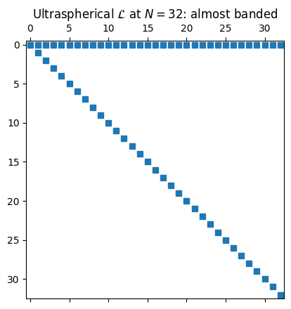

Multiplication operator for variable coefficients¶

For an equation with a variable coefficient like $a(x)\, u'(x) + u(x) = f(x)$, we need one more piece: a multiplication operator $M_1[a]$ that takes the $U$-coefficients of $u'$ and returns the $U$-coefficients of $a\, u'$. We build it in three steps using the Chebyshev recurrence.

Building block. Multiplication by $x$ in the $U$ basis. The identity $x\, U_k = \tfrac{1}{2}(U_{k+1} + U_{k-1})$ (with $U_{-1} = 0$) gives the symmetric tridiagonal

Multiplication by $T_k$. The Chebyshev recurrence $T_{k+1} = 2 x T_k - T_{k-1}$ lifts directly to operators:

Each application of $M_1[x]$ widens the band by one, so $M_1[T_k]$ has bandwidth exactly $k$.

General $a$. If $a(x) = \sum_{k=0}^{d} a_k\, T_k(x)$, linearity gives

a banded matrix of bandwidth at most $d$. A coefficient $a$ with a short Chebyshev expansion produces a narrow operator. The simplest case $a(x) = 1 + x$ has $a_T = (1, 1, 0, \ldots)$ and gives the tridiagonal $M_1[1+x] = I + M_1[x]$.

The full operator. For $a(x)\, u'(x) + u(x) = f(x)$,

an almost-banded operator: dense top row from the boundary condition, banded interior of bandwidth $\max(d, 2)$. The construction extends to any number of dense rows (more boundary conditions) and any short-Chebyshev coefficients.

This is the operator we use in Adaptive QR: Choosing N on the Fly to drive the QR sweep on a genuinely variable-coefficient problem.

Preconditioning for direct solves¶

The ultraspherical operator $\mathcal{L}$ is sparse, but it is not yet well-scaled. The differentiation matrix $\mathcal{D}_0$ has rows growing linearly with the column index — entry $\mathcal{D}_0[k-1, k] = k$, so the $k$-th column of the interior is $k$ times bigger than the first. A direct solve via linalg.solve works, but its forward error inherits a condition number that scales with $N$.

The fix is a diagonal right preconditioner (Olver & Townsend (2013), §4.1). For an order-$\nu$ operator, set

For the first-order problems of this section ($\nu = 1$): $R = \mathrm{diag}(1,\, 1,\, \tfrac{1}{2},\, \tfrac{1}{3},\, \ldots,\, \tfrac{1}{N})$.

The recipe for a direct solve is two lines of bookkeeping.

1. Build $\tilde{\mathcal{L}} := \mathcal{L}\, R$ by scaling the columns of $\mathcal{L}$.

2. Solve $\tilde{\mathcal{L}}\, \mathbf{y} = \mathbf{g}$ as usual, then recover $\mathbf{c} = R\, \mathbf{y}$.

Olver-Townsend prove $\kappa_2(\tilde{\mathcal{L}}) \le 53.6$ for the Dirichlet problem independent of $N$, so the preconditioned solve has the same $O(N)$ cost but a bounded condition number. The same trick works for the streaming QR of Adaptive QR: Choosing N on the Fly: scale columns on the way in and rescale the recovered solution on the way out; the factorisation itself is unchanged.

from math import factorial

def column_scaling(n, nu):
    """Olver-Townsend right preconditioner for an order-nu ODE."""
    R = np.ones(n)
    if nu >= 2 and nu - 1 < n:
        R[nu - 1] = 1.0 / factorial(nu - 1)
    for k in range(nu, n):
        R[k] = 1.0 / k
    return R

# Condition number, with and without preconditioning, on the simplest
# first-order operator L = (b^T; D_0).
print(f"{'N':>5}  {'kappa(L)':>12}  {'kappa(L R)':>12}")
for N in [16, 32, 64, 128, 256, 512]:
    L = ultra_first_order(N)
    R = column_scaling(N + 1, nu=1)
    LR = L * R[None, :]                          # column scaling
    print(f"{N:5d}  {np.linalg.cond(L):12.2e}  {np.linalg.cond(LR):12.2e}")

    N      kappa(L)    kappa(L R)
   16      2.82e+01      3.28e+00
   32      5.65e+01      3.31e+00
   64      1.13e+02      3.33e+00
  128      2.27e+02      3.34e+00
  256      4.53e+02      3.34e+00
  512      9.07e+02      3.34e+00

Without scaling, $\kappa(\mathcal{L})$ grows with $N$. With scaling, the condition number is bounded by a small constant. That is what makes the ultraspherical method well-conditioned in the practical sense, not just sparse.

Physical-Space Collocation: an Alternative¶

The textbook alternative writes everything in the value basis at Chebyshev nodes. Let

be a linear two-point BVP, and let $\mathbf{u} = (u(x_0), \ldots, u(x_N))^T$ be the unknown values at the type-1 Chebyshev nodes. From §5, differentiation at the nodes is $D_N \mathbf{u}$ and $D_N^2 \mathbf{u}$, so the differential operator becomes the matrix

Demanding $L_N \mathbf{u} = \mathbf{f}$ at the interior nodes and replacing the first and last rows with the boundary conditions gives a square linear system to solve.

That is all there is to it: one differentiation matrix, one diagonal multiplication for each coefficient, two row replacements for the boundary conditions.

Worked example¶

Solve $-u'' + (1 + x^2)\, u = f$ on $[-1, 1]$ with homogeneous Dirichlet boundary conditions, manufacturing $f$ from $u_{\mathrm{exact}}(x) = (1 - x^2)\, e^{\sin 5x}$.

Source

def cheb_diff_matrix(N):
    x = np.cos(np.pi * np.arange(N+1) / N)
    c = np.ones(N+1); c[0] = 2; c[N] = 2; c[1::2] *= -1
    X = np.outer(x, np.ones(N+1)); dX = X - X.T + np.eye(N+1)
    D = np.outer(c, 1/c) / dX
    D -= np.diag(D.sum(axis=1))
    return D, x

def solve_bvp(a, b, c, f, alpha, beta, N):
    D, x = cheb_diff_matrix(N)
    L = np.diag(a(x)) @ D @ D + np.diag(b(x)) @ D + np.diag(c(x))
    rhs = f(x)
    L[0, :] = 0; L[0, 0] = 1; rhs[0] = beta
    L[N, :] = 0; L[N, N] = 1; rhs[N] = alpha
    return x, la.solve(L, rhs)

ue = lambda x: (1 - x**2) * np.exp(np.sin(5*x))
def rhs_f(x):
    s, c5 = np.sin(5*x), np.cos(5*x); E = np.exp(s)
    upp = -2*E - 20*x*c5*E + (1-x**2)*((25*c5**2 - 25*s)*E)
    return -upp + (1 + x**2)*ue(x)

a = lambda x: -np.ones_like(x)
b = lambda x:  np.zeros_like(x)
c = lambda x:  1 + x**2

xx = np.linspace(-1, 1, 600)
x16, u16 = solve_bvp(a, b, c, rhs_f, 0, 0, N=16)

fig, (axL, axR) = plt.subplots(1, 2, figsize=(11, 4.2))
axL.plot(xx, ue(xx), 'k', lw=2, label='exact')
axL.plot(x16, u16, 'o', ms=5, label='spectral, $N=16$')
axL.set_title('BVP solution'); axL.legend(); axL.set_xlabel('$x$')

Ns = np.arange(8, 81, 4)
err = []
for N in Ns:
    x, u = solve_bvp(a, b, c, rhs_f, 0, 0, N)
    err.append(np.max(np.abs(u - ue(x))))
axR.semilogy(Ns, err, 'o-')
axR.set_xlabel('$N$'); axR.set_ylabel(r'$\|u_N - u\|_\infty$')
axR.set_title('Spectral convergence')
plt.tight_layout(); plt.show()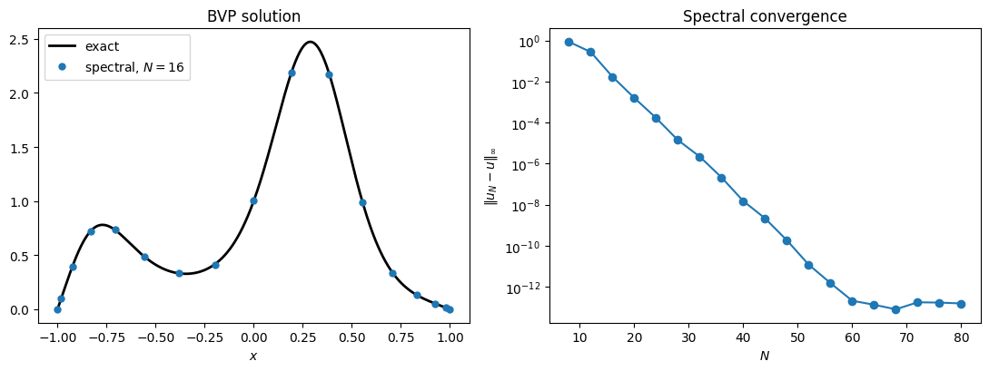

The error halves the digit count between $N = 8$ and $N = 32$. This is geometric convergence, exactly the coefficient-decay result transported through the linear solve.

The conditioning problem¶

Geometric convergence is the prize. The cost is two-fold:

1. Density. $L_N$ is dense, so each solve costs $O(N^3)$ instead of $O(N)$ for a banded system.

2. Conditioning. From §5, $\kappa(D_N^2) \sim N^4$. Backward stability of solve then bounds the achievable accuracy at $\kappa(L_N) \cdot \varepsilon_{\mathrm{mach}} \sim N^4 \cdot 10^{-16}$. For high-order operators (think $u^{(4)}$ in beam equations) the exponent grows: $\kappa(D_N^k) \sim N^{2k}$. Pushing $N$ above a few hundred in double precision is hopeless.

The two costs are visible side by side: the dense physical-space $D_N$ next to the almost-banded ultraspherical $\mathcal{L}$.

Source

N = 32
D_phys, _ = cheb_diff_matrix(N)
L_ultra = ultra_first_order(N)

fig, axes = plt.subplots(1, 2, figsize=(10, 4.5))
axes[0].spy(D_phys, markersize=3)
axes[0].set_title(f'Physical-space $D$: dense, $N = {N}$')
axes[1].spy(L_ultra, markersize=6)
axes[1].set_title(r'Ultraspherical $\mathcal{L}$: almost banded')
plt.tight_layout(); plt.show()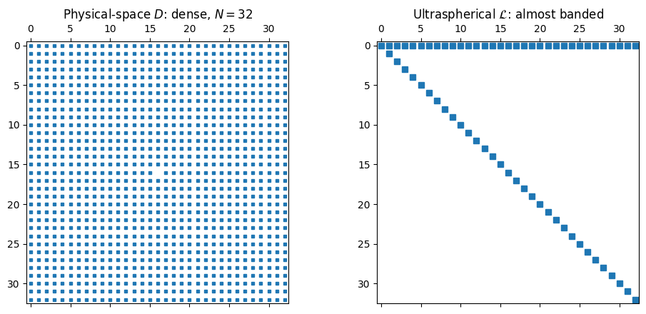

Physical-space collocation is the right tool when $N$ is moderate and the operator is well-conditioned. For stiff or high-order problems, or when $N$ has to grow large, the ultraspherical formulation pays off.

Higher-Order Operators¶

The construction above generalises cleanly to any order of derivative. A second derivative $u''$ lives in $C^{(2)}$, requiring a sparse differentiation map $\mathcal{D}_1: U \to C^{(2)}$ and a conversion $\mathcal{S}_1: U \to C^{(2)}$. A multiplication operator $M_2[a]$ acting on $C^{(2)}$-coefficients is built by the same three-term recurrence as $M_1[a]$, with the appropriate Gegenbauer recurrence in place of the Chebyshev one. For an equation of order $k$, the discretisation lives in $C^{(k)}$ and the resulting operator is again almost banded, with bandwidth determined by the differentiation order and the smoothness of the variable coefficients. The full theory, along with the analysis of conditioning and the optimal $O(N)$ solver, is in Olver & Townsend (2013).