Ridge Functions and Universal Approximation

Why we care: functions on $\mathbb{R}^d$ in practice¶

The input $x \in \mathbb{R}^d$ is just a list of $d$ numbers, and that covers most of the real-world objects we want to compute with:

• Images: pixel intensities, $d \sim 10^4$ to 10⁶.

• Text: word or sentence embeddings, $d \sim 10^2$ to 10⁴.

• Molecules: atomic positions, charges, and types, $d \sim 10^2$ for small molecules.

• Games and control systems: the state of a board, robot, or vehicle at one moment in time.

• Models: the parameters of a physical or financial model whose outcome we want to predict.

The function $f: \mathbb{R}^d \to \mathbb{R}$ (or $\mathbb{R}^m$) we want is then “image $\to$ class label”, “sentence $\to$ translation”, “molecule $\to$ binding energy”, “board state $\to$ best move”, “model parameters $\to$ option price”. None of these are available in closed form, and the input dimensions are firmly outside what tensor-product Chebyshev or any other deterministic basis can handle. The next page makes that obstacle quantitative (the curse of dimensionality) and shows under what hypothesis a neural network gets around it (Barron’s theorem). The current page builds the basis (ridge functions), shows it can represent any continuous target (universal approximation), and demonstrates a 1D failure mode that flips when $d$ is large.

A neural network as a basis expansion¶

A one-hidden-layer network is

with $x \in \mathbb{R}^d$, weights $w_k \in \mathbb{R}^d$, biases $b_k$, output coefficients $a_k$, and a fixed non-linearity $\sigma$. Stacking the $w_k^\top$ as rows of a matrix $W \in \mathbb{R}^{n \times d}$ gives the matrix form

with $\sigma$ acting elementwise.

Each term $\sigma(w_k \cdot x + b_k)$ is a ridge function: a 1D function $\sigma$ depending on $x$ only through $w_k \cdot x + b_k$, extruded along the $(d-1)$ directions perpendicular to $w_k$. A network is a sum of $n$ such ridges; $w_k$ controls the direction, $b_k$ shifts it, $a_k$ scales it.

Compare with a Chebyshev expansion $f_n(x) = \sum c_k T_k(x)$. Both are linear combinations of $n$ basis functions. The Chebyshev basis $\{T_k\}$ is fixed; the ridge basis $\{\sigma(w_k \cdot x + b_k)\}$ is parameterised by $(w_k, b_k)$ that we can choose.

A 1D ridge network: evaluation, differentiation, integration¶

In one variable a ridge is just a shifted, scaled copy of $\sigma$: $\phi_k(x) = \sigma(w_k x + b_k)$ with $w_k, b_k \in \mathbb{R}$. The basis is parameterised but each basis function is something we can draw on a single axis. Before doing any algebra, look at it.

What a ridge basis looks like¶

Three panels. The left shows three single ridges with different $(w, b)$. The slope at the inflection point is $w/4$ for $\tanh$, so $|w|$ controls how fast the ridge transitions from one saturation level to the other; the sign of $w$ flips left and right; $b$ shifts the inflection point to $x = -b/w$. The middle panel overlays a few $a_k\,\sigma(w_k x + b_k)$, dashed unscaled and solid scaled, to show how $a_k$ rescales each individual ridge. The right panel adds them up and overlays a target.

Source

import numpy as np
import matplotlib.pyplot as plt

sigma = np.tanh
xs = np.linspace(-2, 2, 400)

fig, axes = plt.subplots(1, 3, figsize=(11, 3.2))

# Panel 1: three single ridges
ax = axes[0]
for w, b, label in [(1, 0, r"$w=1,\ b=0$"),
                    (4, 0, r"$w=4,\ b=0$"),
                    (-2, 1, r"$w=-2,\ b=1$")]:
    ax.plot(xs, sigma(w * xs + b), label=label)
ax.set_title(r"Single ridges $\sigma(wx+b)$")
ax.legend(fontsize=8, loc="lower right")
ax.set_xlabel(r"$x$"); ax.grid(alpha=0.3)

# Panel 2: scaled vs unscaled
ax = axes[1]
params = [(3, -1, 1.0), (-2, 0.5, -0.7), (1.5, 1, 1.3)]
for w, b, a in params:
    ax.plot(xs, sigma(w * xs + b), '--', alpha=0.45)
    ax.plot(xs, a * sigma(w * xs + b), '-')
ax.set_title(r"Scaled ridges $a_k\,\sigma(w_k x+b_k)$")
ax.set_xlabel(r"$x$"); ax.grid(alpha=0.3)

# Panel 3: sum vs target
ax = axes[2]
target = lambda t: np.sin(2 * np.pi * t) * np.exp(-0.5 * t**2)
rng = np.random.default_rng(0)
n = 30
ws = rng.normal(scale=4, size=n)
bs = rng.uniform(-3, 3, size=n)
V = sigma(np.outer(xs, ws) + bs)
y = target(xs)
a, *_ = np.linalg.lstsq(V, y, rcond=None)
ax.plot(xs, y, 'k-', lw=2, label="target")
ax.plot(xs, V @ a, '--', lw=1.5, label=f"sum, $n={n}$")
ax.set_title(r"Sum $\sum_k a_k\,\sigma(w_k x+b_k)$")
ax.legend(fontsize=8); ax.set_xlabel(r"$x$"); ax.grid(alpha=0.3)

plt.tight_layout()
plt.show()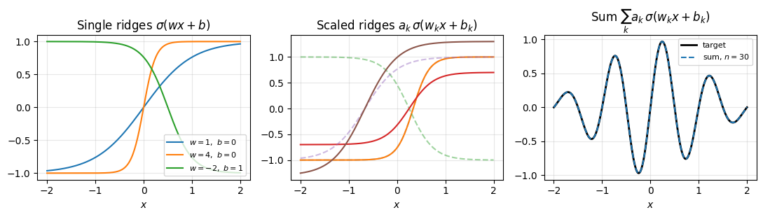

The takeaway: each ridge contributes one bend, localised to a region of width $\sim 1/|w_k|$ around $x = -b_k/w_k$. Outside that region the ridge is essentially constant and adds nothing. Contrast with Chebyshev, where every $T_k$ oscillates across the entire interval $[-1, 1]$. Ridges are local, polynomials are global. This single fact drives the difference in behaviour in high dimensions: a $d$-variable ridge is a 1D bump pulled along $d-1$ flat directions, so its cost does not multiply with $d$, while a tensor-product basis of global polynomials does.

Random features: the linear case¶

The simplest way to fix $(w_k, b_k)$ is to draw them randomly from a probability distribution, for instance $w_k \sim \mathcal{N}(0, \sigma^2 I)$ and $b_k \sim \mathcal{U}(-c, c)$. Once drawn, the weights are frozen and only $\{a_k\}$ varies; every operation becomes linear in the coefficient vector $a$, and the ridge basis is a fixed basis like $\{T_k\}$. This is the random-features view of a one-hidden-layer network: no training, no gradient descent, just a random draw followed by a single linear solve.

The random draw raises two questions we defer to the next page: which distribution to sample from (Fourier inversion picks out the right one) and what does random sampling buy quantitatively (the draw is a Monte Carlo sample, with the dimension-free $\sqrt V/\sqrt n$ rate). Both are answered in §Barron. For now any concrete distribution suffices to demonstrate the construction.

We come back to the trained case at the end, where the random draw is replaced by gradient descent on $(w, b)$.

Evaluation¶

$f_n(x) = a^{\!\top} \phi(x)$ at a point. For a batch $x_1, \ldots, x_N$, this is $f_n = V a$ with $V_{jk} = \phi_k(x_j)$. Cost $O(Nn)$, the same shape as Chebyshev’s value-from-coefficient map.

Differentiation¶

$\phi_k'(x) = w_k\, \sigma'(w_k x + b_k)$, so

The coefficient map is $a \mapsto W a$ with $W = \mathrm{diag}(w_k)$, expressed in the related basis $\sigma'$. Like Chebyshev: differentiation maps $T_k \to U_{k-1}$ to a different family, and a recurrence converts back. For ridges we evaluate in the $\sigma'$-basis directly.

Integration¶

If $\Sigma' = \sigma$ then $\int \phi_k = \Sigma(w_k x + b_k) / w_k$. For $\sigma = \tanh$, $\Sigma = \log\cosh$. The definite integral is

A linear functional with precomputed moments, identical in shape to the Chebyshev integration construction.

Fitting¶

Given data $\{(x_j, f(x_j))\}_{j=1}^N$ and the frozen weights from above, the coefficients $a$ minimise the empirical loss

a linear least squares problem in $a$. With Chebyshev nodes for $\{x_j\}$ and the $T$-basis the matrix $V$ is structured and a DCT solves it in $O(N \log N)$. With random ridges no such structure, but the standard QR-based least-squares solver from §Least Squares is still cheap, and there is no non-convex search.

The empirical loss is itself a Monte Carlo estimator of the population loss

provided the data points $\{x_j\}$ are drawn iid from $\mu$; $\hat L$ is unbiased for $L$ and its standard deviation around $L$ decays as $\sqrt V/\sqrt N$ (see the Monte Carlo notebook for the standard rate). So the random-features network is doing two things at once: sampling weights, and estimating an integral (the loss) from samples. The first piece is what §Barron makes principled.

The trained case¶

If we let $(w_k, b_k)$ vary too, the loss

is non-convex. To see why, recall the basis matrix $V \in \mathbb{R}^{N \times n}$ from the fitting section above: $V_{jk} = \sigma(w_k \cdot x_j + b_k)$ is the $k$-th basis function evaluated at the $j$-th data point. With $(w, b)$ frozen, $V$ is a fixed matrix and $\hat L = \tfrac{1}{N}\|Va - f\|_2^2$ is quadratic (hence convex) in $a$. Once we let $(w, b)$ vary, $V$ depends nonlinearly on $w$ through $\sigma(w_k \cdot x_j + b_k)$, the loss loses its quadratic structure, and many local minima appear. There is no closed-form solver. We descend.

Stochastic gradient descent¶

Vanilla gradient descent updates $\theta_{t+1} = \theta_t - \eta\,\nabla \hat L(\theta_t)$ with $\nabla \hat L = (1/N)\sum_j \nabla \ell_j$ and $\ell_j = (f(x_j) - f_n(x_j;\theta))^2$. Each step costs $O(N)$ work; for $N$ in the millions this is unaffordable.

Stochastic gradient descent (SGD) replaces the full sum with a random mini-batch $\mathcal{B}_t \subset \{1, \ldots, N\}$ at each step (sizes 32 to 128 are typical):

Per-step cost drops to $O(|\mathcal{B}|)$. The mini-batch gradient $\hat g_t$ is a Monte Carlo estimator of the full-batch gradient: unbiased, with variance $O(1/|\mathcal{B}|)$. So in expectation each step does what gradient descent would; in any individual step the direction is noisy. In practice the step size $\eta$ is adapted per parameter using moving averages of $\hat g_t$ and $\hat g_t^{\,2}$; this is Adam, the standard default.

The full training loop:

The “backward pass” step is just calculus: differentiate the loss with respect to each parameter. For a one-hidden-layer ridge network everything is fully explicit, which makes the training loop entirely concrete. For deeper networks the same chain-rule pattern is what backpropagation automates.

Let $\delta_j = f(x_j) - f_n(x_j; \theta)$ be the residual at sample $j$, and $\ell_j = \delta_j^2$. Differentiating:

The mini-batch gradient is the average of these over $j \in \mathcal{B}_t$. Libraries (PyTorch, JAX) compute these automatically by reverse-mode automatic differentiation, but for a one-layer net you can write them by hand and verify.

The universal approximation theorem¶

The 1D story above shows ridges are a basis we can compute with: we can evaluate, differentiate, integrate, and fit, exactly as we did with $\{T_k\}$. The first question to settle, before any quantitative rate, is whether this basis is flexible enough to represent every continuous function. That is the density question, and is what universal approximation answers.

Stone–Weierstrass already gives polynomial density in $C(K)$ for compact $K \subset \mathbb{R}^d$, so “any continuous function in any dimension is approximable by polynomials” was a solved problem. Cybenko (1989) and Hornik (1991) added that ridge functions are also dense, under a hypothesis on $\sigma$ called discriminatory.

The condition says: no signed measure can be invisible to every ridge function with activation $\sigma$. Equivalently, the closed linear span of $\{\sigma(w \cdot x + b)\}_{(w,b)}$ in $C(K)$ has no non-trivial annihilator, which by Hahn–Banach means the span is dense.

A self-contained proof (Hahn–Banach plus a Fourier argument that continuous sigmoidal activations are discriminatory) is on this companion site for MATH 725. The two activations that dominate in practice both satisfy the hypothesis:

• tanh / sigmoid: continuous sigmoidal ($\lim_{t \to -\infty}\sigma(t) = 0$, $\lim_{t \to \infty}\sigma(t) = 1$), discriminatory by Cybenko’s Lemma 1. Bounded and smooth, gradients vanish in the saturation regions.

• ReLU, $\sigma(t) = \max(0, t)$: discriminatory under Hornik’s extension, which only requires $\sigma$ to be non-polynomial. Piecewise linear, unbounded, cheap; the modern default.

A first experiment: fitting $\sin(2\pi x)$¶

Train a width-20 network with $\tanh$ on $\sin(2\pi x)$ over $[-1, 1]$. After 2000 Adam steps the network reaches $\sim 10^{-2}$ pointwise error. The adaptive Chebyshev chebfit_adaptive from A Chebyshev Toolbox: Doing Linear Algebra with Functions reaches machine precision on the same function with about 20 coefficients, in one DCT. Both get arbitrarily close to $\sin(2\pi x)$; the network needs thousands of gradient steps and still plateaus at 10^-2. In 1D the network is strictly worse than what we already have. The picture flips in high $d$. Demo 1 of the companion notebook.